Hello readers, for this article I am going to explain my approach to create a forecast system of the French (metropolitan) energy consumption. This kind of problematics is more or less related to part of my job at EDF Energy but this works has been done in my free time to complete my machine engineer nanodegree of Udacity.

In this article, there will be a description of the data used for this project, an explanation of the approach used to make a daily forecast of the consumption and the half hourly version.

Exploration of the dataset

In this case, the data to create the model are from:

• RTE, the energy network manager in France they have created an open data platform to access different datasets on the network
• The GEOFLA dataset that give you informations on the number of inhabitants in the city and the area
• Weather underground. I have to scrap this data source from the website (I focus my scraping on the weather stations from the airports) and I pick the weather stations that have enough data during the period measured by RTE.I focus my data analytics on the outdoor temperature and the wind speed.

For the weather condition, I choose to create a national weather dataset where basically each region has his weather station associated , these stations are weighted by the number of people that are in this region (this information is coming from the GEOFLA dataset).To make the data analysis, I choose to convert the average power consumed from RTE in energy (in MWh).

In the following figure there is an illustration of the average energy consumed in France for the past years.

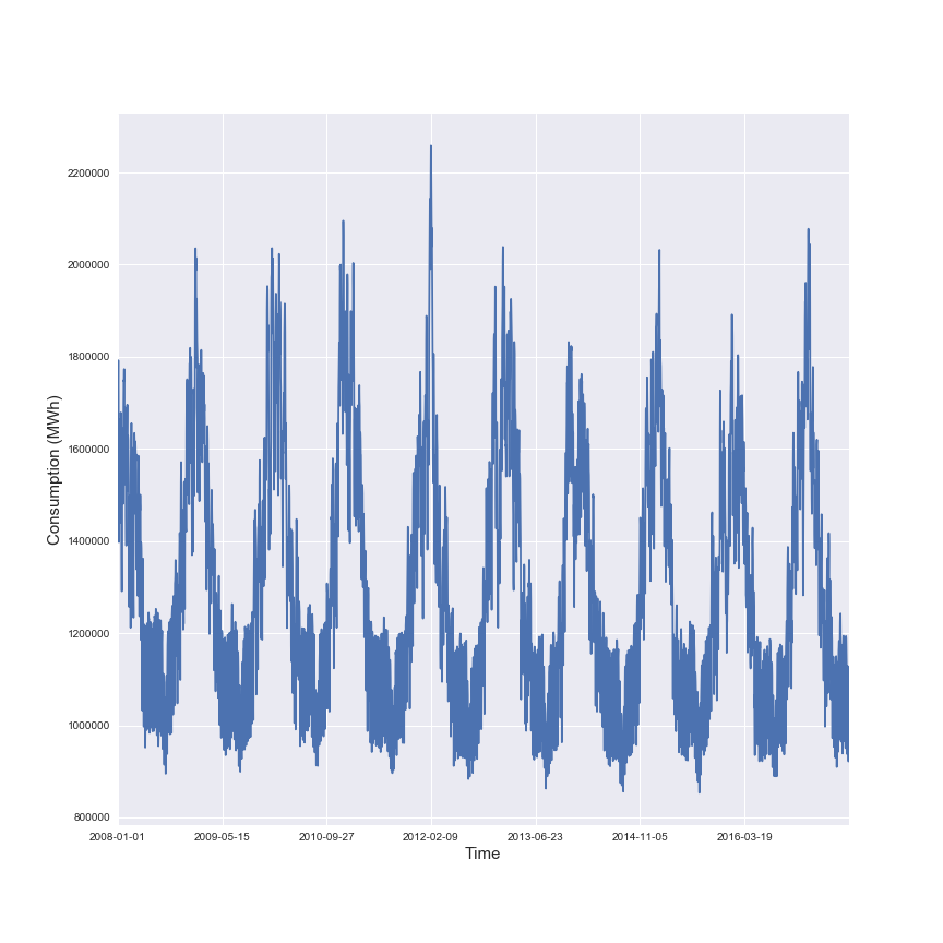
This figure illustrates the seasonality in the energy consumption in France.

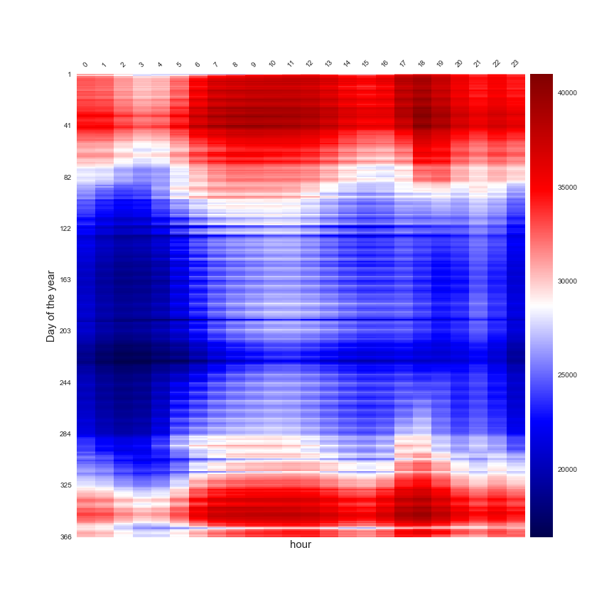
After that to make the forecast at a daily scale, I have to aggregate the data. In the following figures, there is a representation of the daily data aggregated at different scale in a heatmap.

A study of the hourly effect in function of the day of the year

A study of the consumption of the month of the year and the day of the week.

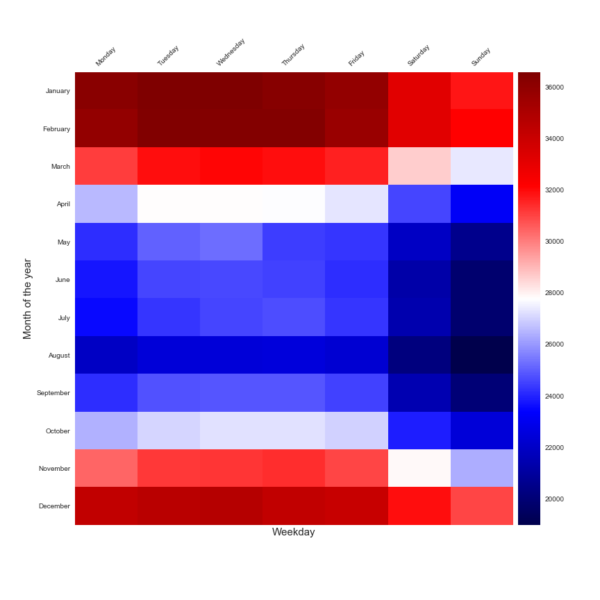
This two figures are perfect to illustrate that the daily consumption is linked to the moment of the year and the day of the week. But this insight are not enough to create a forecast model, a very popular approach that is used to make a forecast of the energy consumption is the study of the daily consumption in function of the average daily outdoor temperature. This technic is called PTG for Power Temperature Gradient and you can find a lot of publications that are based on this approach.

In the following figure there is a representation of this model used for the forecast.

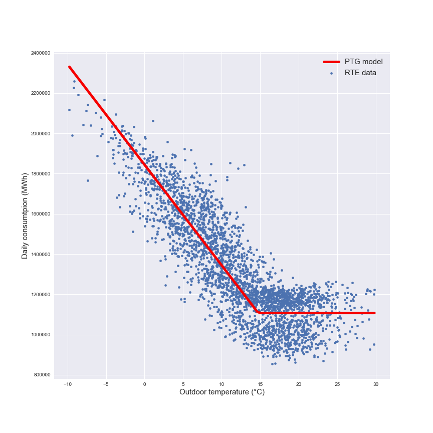
The model is a piecewise regression with a winter part represented by the linear regression (that’s included the heating needs and the appliances) and a summer part with the constant part (only the appliances). This model will be the reference model for the next part.

Daily forecast

To create the model, the dataset will be split between training set and test set, the selection of the samples for the sets will be randomized. That’s representing:

• 2337 samples for the training set
• 585 samples for the test set

This is a regression problem, so the following models from scikit learn are going to be tested:

• Polynomial regressor
• Random forest regressor
• Decision tree regressor
• K-nearest neighbours
• Neural network MLP regressor

This is a personal selection of different models and there is plenty of other models to try but for a start I think that was enough. I have to tune the different models and find the best parameters to used, I used a k-fold approach on the training set (I created ten folds) to test the different parameters. I invited you to check my report to see the choices done on the parameters for the different models.

To test the impact of the input in the models, I tested different inputs:

• only outdoor temperature
• outdoor temperature and wind speed
• outdoor temperature and month of the year and day of the week

To facilitate the usage of the inputs I have to normalise the sets. To assess the accuracy of the model I used the r²score metric that is used for the regression problem. But this metric is not enough to assess the quality of the algorithm, the second metrics that I will use is the time to create the model. In the following table there is the evolution of the r²score in function of the model used.

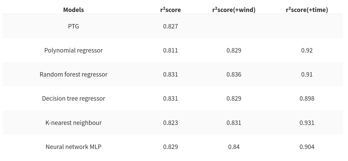
This table permits to give the following conclusions:

• The PTG is quite a good model, for an only outdoor temperature based model the score is good but the tree based model offers and the neural network offer good results too
• the addition of the wind speed improves the score but the gain is very small
• the addition offer an interesting gain to the score for every model tested

But as I said previously the r²score is not enough, in the following table there is the time to create the model in the case of the addition of the time features to the initial inputs.

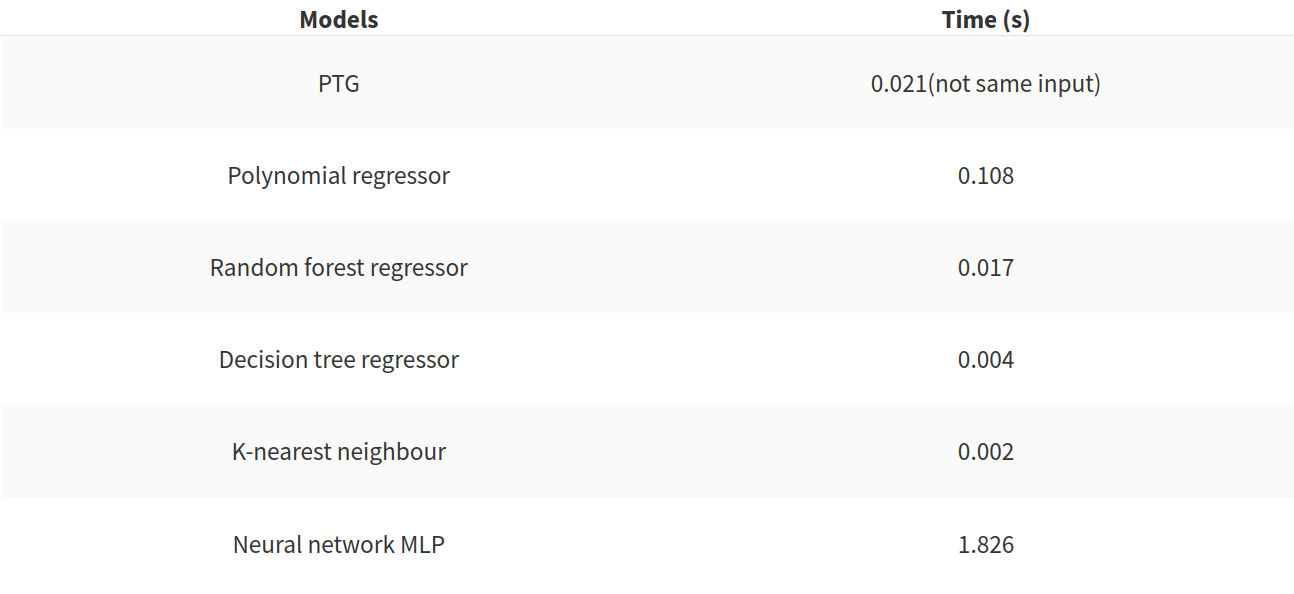
This table is illustrating that the PTG has good performance, and that the neural network is very bad in term of speed. The polynomial regressor should be avoided too.But this two metrics are not enough to evaluate the efficiency of the models. The impact of the size of the training set should be studied. In the following figure, there is an illustration of the impact of the training set.

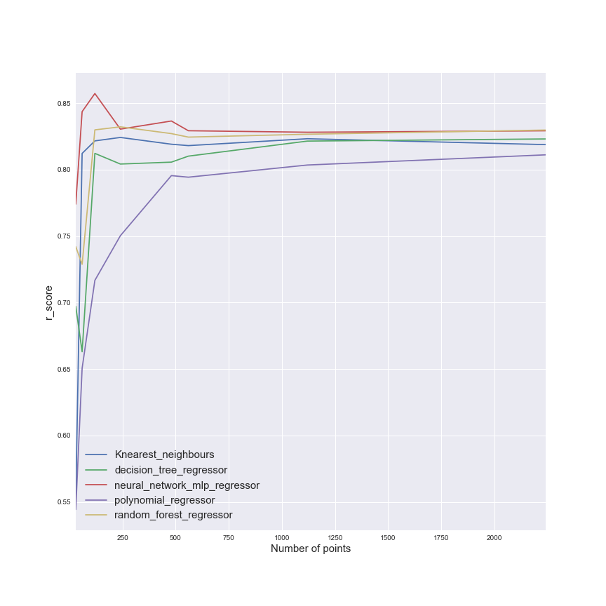
This figure show us that the size of the training set has a clear impact on the polynomial regressor, so other models seems less impact (the neural network show good efficiency quite quickly).

Half hourly forecast

For this part, we will used all the results found previously (the used of the time features essentially). I will test the same models than for the daily forecast and used the same metrics.

My benchmark model will be the ARIMA model.this model is quite popular to forecast time series (but need to not randomized the sets).These sets are composed of:

• 112176 samples for the training set
• 28080 samples for the test set

In my problem the result of the model are bad. In the following table there is summary if the result of the benchmark model and the other models tested.

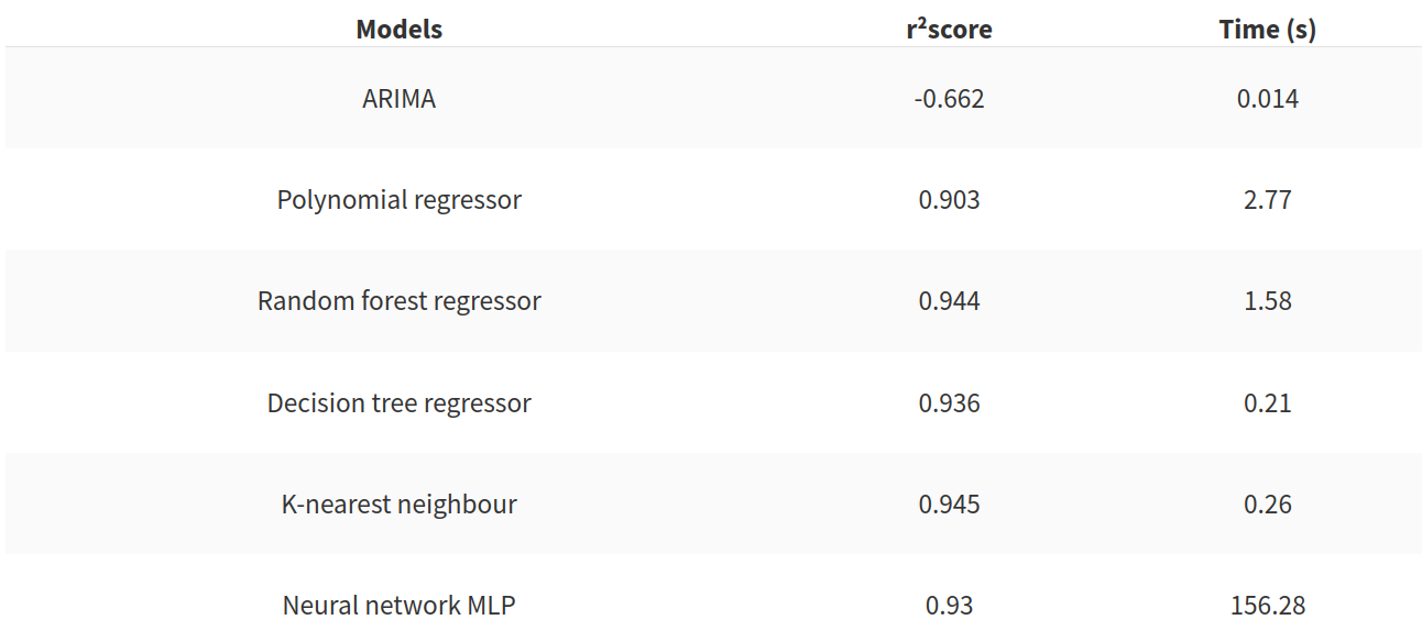
This final table, show us that the benchmark model is quite easy to beat. The neural network is very slow to construct but two models seems very good to used for our problem:

• the decision tree regressor
• the K-nearest neighbour

Conclusion

This work was used to complete my nanodegree, this is my approach, not the only one and I think there is a lot of things to try like a deep learning approach or a reinforcement learning one for example.

I invite you to used the datasets of this project to try to create your own (better?!) model and if you have any comments write it below.