Hello, the goal of this article is to offer a clear description of the dataset that I uploaded in November 2017 on Kaggle followed by some insights on the dataset.

Description of the dataset

To better follow the energy consumption, the government wants energy suppliers to install smart meters in every home in England, Wales and Scotland. There are more than 26 million homes for the energy suppliers to get to, with the goal of every home having a smart meter by 2020.

This roll out of meter is lead by the European Union who asked all member governments to look at smart meters as part of measures to upgrade our energy supply and tackle climate change. After an initial study, the British government decided to adopt smart meters as part of their plan to update our ageing energy system.

In this dataset, you will find a refacted version of the data from the London data store, that contains the energy consumption readings for a sample of 5,567 London Households that took part in the UK Power Networks led Low Carbon London project between November 2011 and February 2014. The data from the smart meters seems associated only to the electrical consumption.

To have an easier dataset to manipulate, different transformations have been applied on the dataset:

• Collection of all the data from a specific household in the same file (that was not the case in the original dataset)
• People from the same ACORN group are on the same file

The original and clean dataset can be find in the halfhourly_dataset zip file and one file looks like this snapshot.

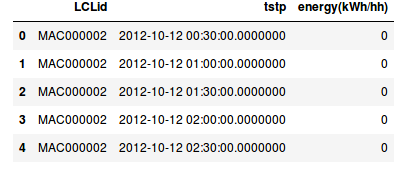
Preview of the half hourly data

As you can see the dataset is quite easy to manipulate with:

• LCLid that corresponds to the household id
• tstp the timestamp of the measure
• energy(kWh/hh) the energy consumes in the past 30 minutes in kWh

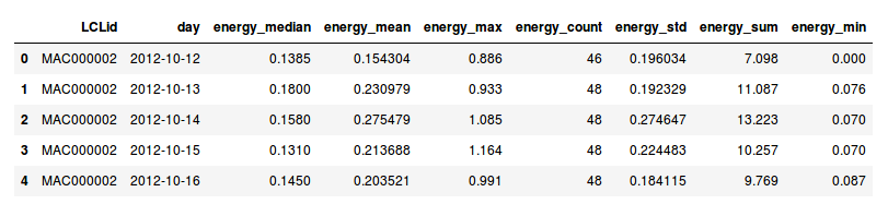
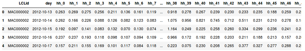
But to make the life easier for the user of my dataset, I created two others zip files that contains some pre-process data:

• the daily_dataset that contains daily informations on the consumption of the households

• the *hhblock_dataset* that contains the transpose data of a day for one household (as an array) with for example the hh_0 column is the consumption between 00:00 and 00:30

######

This is an overview of  all the data from the smart meter, but to facilitate the exploration there is a table that stored all the households and their associated files (informations_households.csv).

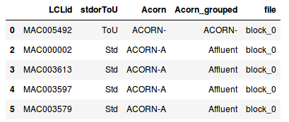
In this table, there is:

• LCLid that correspond to the household id
• stdorToU the kind of tariff applied (ToU the dynamic tariff in function of the days or Std the classic fixed tariff)
• Acorn the ACORN group associated, that categorises the household
• Acorn_grouped this is another more global classification of the ACORN (fusion of different ACORN groups)
• file name of the file in the different zip files where you can find the data of the household

All these informations are from the original dataset but to complete the informations available to make other study there is an addition of some new datasets:

• acorn_details.csv : that contains the index for multiple parameters in comparison of the national (that have an index of 100)

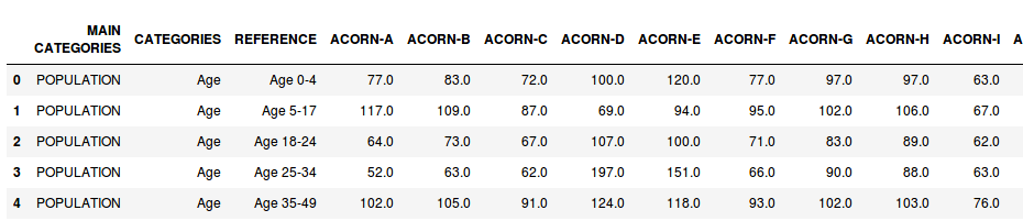
Preview of the details on the ACORN groups

• uk_bank_holidays.csv : the bank holidays for the period of the study

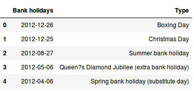
Preview of the details on the bank holidays

• weather_daily_darksky.csv : the daily informations on the weather from darksky at London during the study

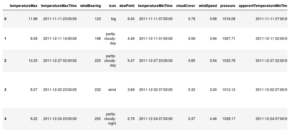
Preview of the daily weather informations

• weather_hourly_darksky.csv : the hourly informations on the weather from darksky at London during the study

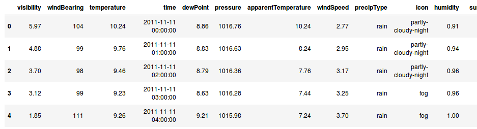
Preview of the hourly weather informations

This first part offers a general overview of the content of the dataset, it’s time now to obtain a clearer vision on the data from the smart meter.

Exploration of the dataset

Selection of the households

First step on this study is to find the best period to make the comparison. In my previous article on the electrical consumption in France there was a seasonal effect so a great period to study will be at least one year of data. In the next figure there is an illustration of the count of households with data (the 48 timestamps in the day) per day of the study.

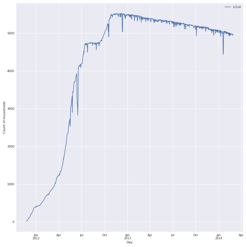
Notes : There is clearly an increase of the number of available households since the start of the study in end 2011, the peak is reach in 2013. A good period for our study could be 2013 (and i choose this one). But it’s now important to know the distribution of the available days for this period in the households of the experiment, in the following figure there is a representation of this distribution in a boxplot.

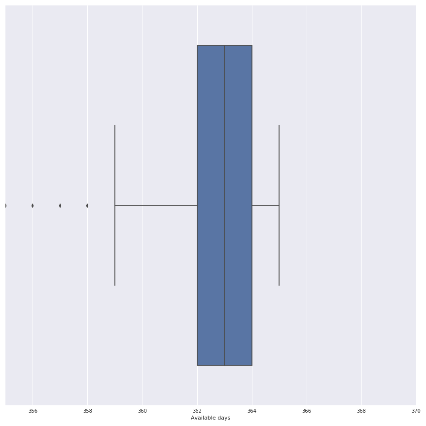
The decision has been done to use the Households that possess at least 357 days, so on the original dataset that represents a lost of 632 households on the 5566 available in the dataset that’s totally acceptable.

Overview of the panel

One of the first realisation is to display the average consumption per day of these households during the year of 2013, in the following figure there is the average global consumption of these households during the period.

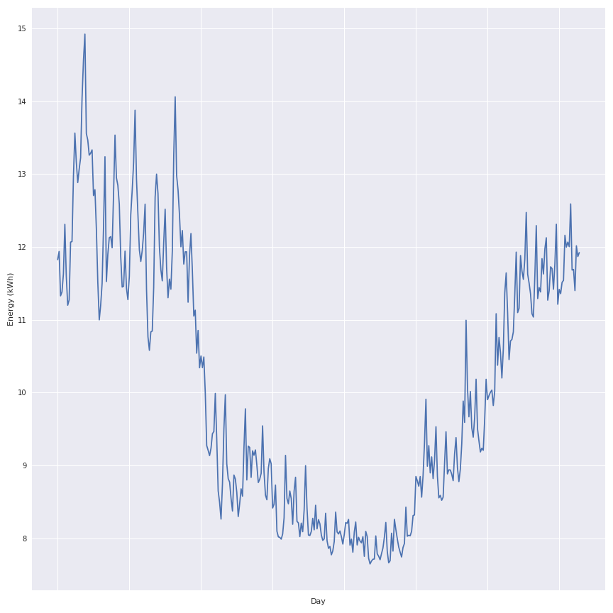
Notes : This is obvious that there is a link between the electrical consumption and the day of the year (same result than in my previous article). The seasonal effect is very clear so in this panel there is a lot of people that are using the electricity as an heating source. If the average daily outdoor temperature and the total daily consumption of the panel are crossed, the following figure display the relation:

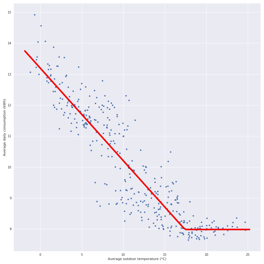
This general observation offers a clear vision that the PTG (The red plot) from the previous article can be calculated for each household.In the following figure, there is a representation of the daily consumption and the PTG associated to this household (and their r² score).

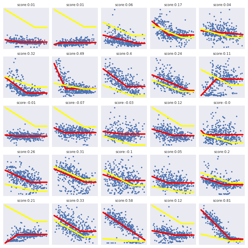
Notes : This is a good illustration that for some households the r² score is working great (this household should have a electric system) but for some households it doesn’t work at all. The general model issued from the average daily consumption (the yellow curve) illustrates that average daily consumption doesn’t represent the general behaviour of the households.In the folowing figure there is the scatter plot of the pivot temperature in function of the r² score.

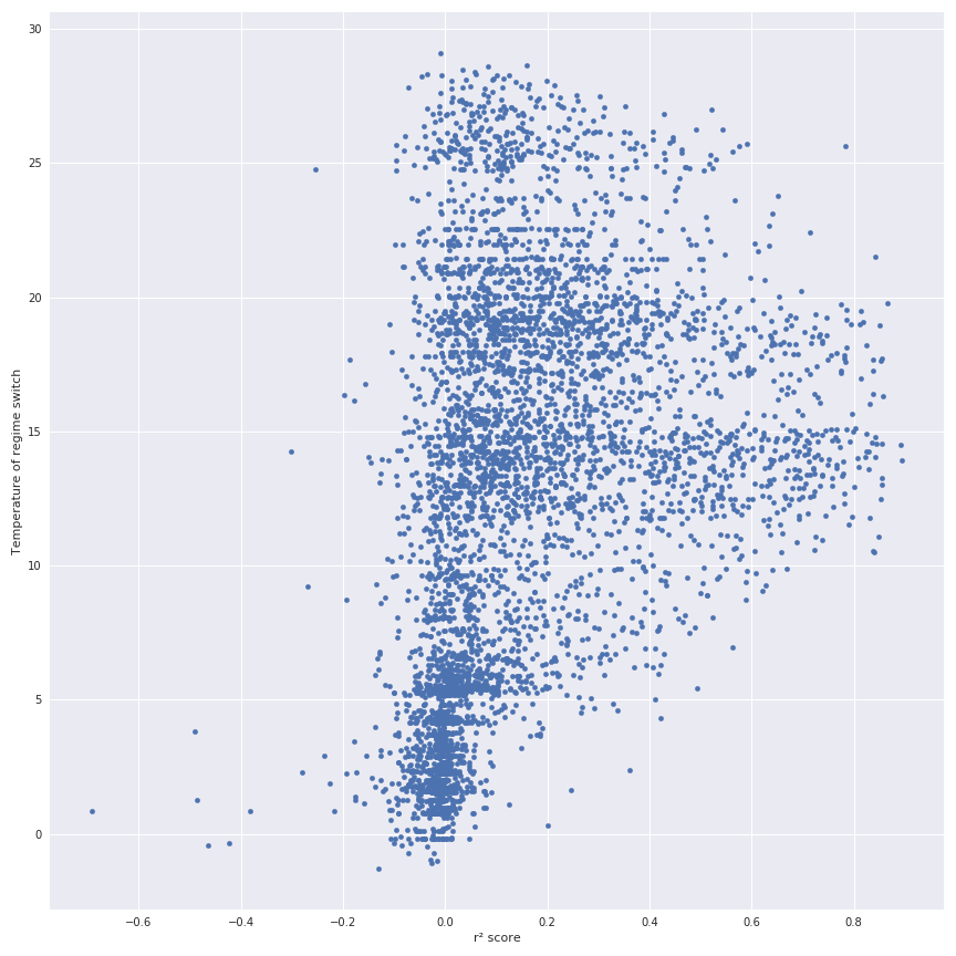
Another way to identify the households that have an electric heating system could be to compare the average consumption during the winter and the summer and make a simple ratio between these two consumptions.The data have been crossed with the informations of the households, and there is an extract of the new dataset.

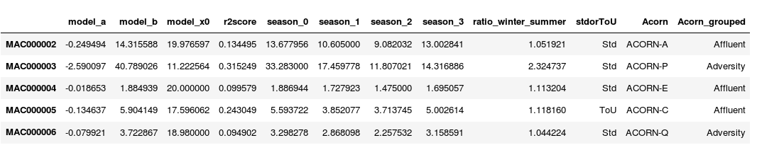
In this dataframe, there is:

• model_a the slope of the ptg model (in the winter part)
• model_b the intersection of the ptg models
• model_x0 the temperature of regime switch
• r2score the r² score of the ptg model on the household
• season_0 the average consumption in winter
• season_1 the average consumption in spring
• season_2 the average consumption in summer
• season_3 the average consumption in autumn
• ratio_winter_summer the ratio of the consumption winter/ration_winter_summer
• stdorToU the type of tariff
• Acorn the ACORN group
• Acorn_grouped tha aggregated ACORN groups

There is a serious amount of data to cross so in the following figure there is a pairplot that cross all this data andfilter thme in function of the Acorn_grouped.

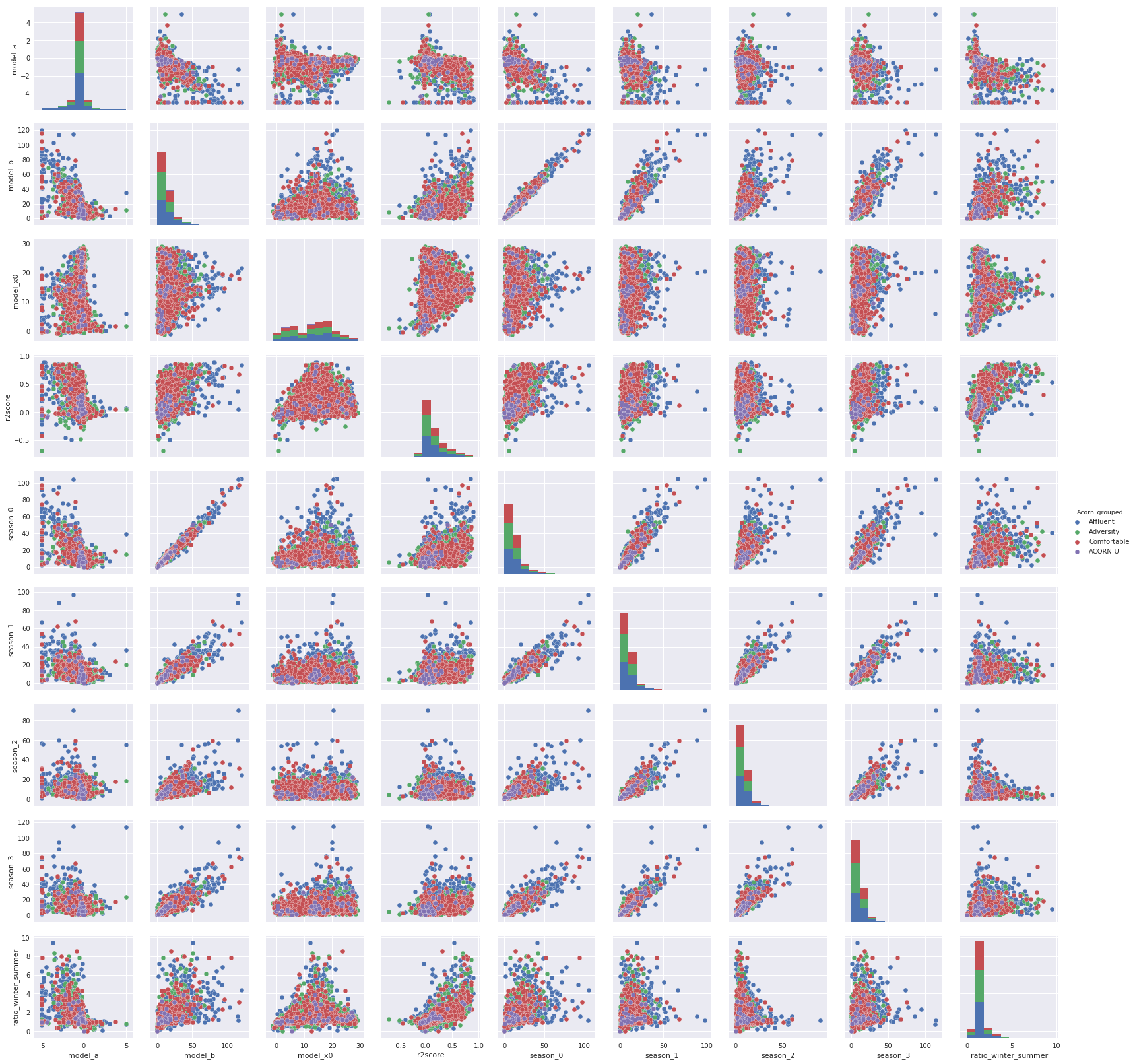
Notes : There is no obvious relation between all this index that defined the households except between the season_0 and the model_b but this two are winter related so that’s normal.But there is no link between these indexes and the Acorn_grouped, the result is similar with the Acorn, that’s a little bit disappointing.

Next steps

As you can see this first exploration of the dataset has highlighted some characteristics of the electrical consumption in London like the influence of the weather in this consumption but there is a lot more things to do on this dataset. Some ideas for future analytics:

• Cross the ACORN data and the smart meter data
• Try to forecast the consumption of the different households
• Add new datasets like:
• EPC data from London
• extra data on London like some underground or train strike during the period
• Make some clusterings in the households data and the energy profiles, as you can see in the following heatmap there is a “pattern” in the total consumption of these households.

You can find all the code to make this article in this GitHub repo