Tune your machine learning workflow with weights and biases, mljar automl, hyperopt, shapash and evidently

I wanted to write for a few weeks around ml/ds libraries that I have on my backlog of things to try. One article per library was maybe too much (and not very dense), so I decided to merge my tests on one article for one use case to test them and make a quick summary on it.

In this article, you will have a quick test (in shotgun) around the following libraries:

I will apply these libraries in a straightforward use case (and my classic use case to test libs) and give some feedback.

All the code to feed this article can be found in this Github repository.

ML setup

In this section, there will be a description of the use case used to test these libraries. My use case is a legacy from my MOOC that I did in 2016 on Udacity, and it’s around forecasting France’s daily electrical consumption; you can find more details on this experiment in this article.

To sum up this article, there are few key points:

Electrical consumption is very dependent on the season (electrical heating is mainly used in France)
People seem to consume more electricity on a Sunday/Saturday than on a weekday.

Based on that, I just rebuild the use case with fresher data from :

Electrical consumption from the rte portal, I made a dump until the 1st January (and aggregate the data at the daily level)
Weather data from the NASA POWER data source focus on the 11 biggest cities and the minimum, average, maximum temperatures at 2 meters (deg Celsius) plus the total precipitation (mm)

From the weather data, I built four features that are a weighted version of these features based on the cities population; you can found the ETL in this notebook.

In terms of preparation, I built :

Training set + testing set that is 80% and 20% of the data between 2015-2020 pick randomly
2020 dataset that are the data from the year 2020

This project aims to see how we can build a good predictor of energy consumption (and how to do it efficiently with these libraries).

Build baseline models with MLJAR automl

One of the first steps to build a predictor is to build baseline models that are easy to put in place and a good starting point to build a better predictor. For this project, the principal evaluation metric will be the RMSE. These first baseline models are going to be :

Random predictor (pick a value between the minimum and maximum of the training set period randomly)
Less random predictor (pick a value between the minimum and maximum a subset of the training set based on the day of the week and the month)
PTG: From the literature, a piecewise regression based on the outdoor temperature is doing a good predictor (so I built three versions based on the min, mean, max weighted temperature)

Finally, and that was the point of this section, another approach to build baseline models that can take maybe more time but will be more challenging is to used automl libraries to create these models. For the ones that are perhaps not familiar with this concept, there is an excellent article by Bojan Tunguz on the subject.

Still, it’s to let an ML library doing some research and test on a dataset to build models, there is plenty of libraries to do this (H20 automl, auto-sklearn, autokeras) but the one that I want to highlight is MLJAR autoML.

They have multiple aspects to this package, but their authors made a nice infographic to explain the features.

You can found in my repository the part that I put in the palace to build a baseline model with mljar (notebook and report), but for me, the critical points on this package are:

Easy to use, really a few lines of code are used to make it work

  automl = AutoML() # mode=Explain, Perform, Compete
  automl.fit(X_train, y_train)
  predictions = automl.predict(X_test)
  rmse = mean_squared_error(y_test, predictions, squared=False)
  evaluation_metrics.append({'model' : 'mljar-bm', 'rmse' : rmse})
  print('RMSE on the test-set:', rmse)

Explainability of the models produced by the system is available and are stored in a local directory (put a sample of the outputof the automl in the repository)
The automl element can be configured with various modes: Explain, perform, compute optuna. This mode can be select in the function of the time to build the model, and the level of explainability expected (cf documentation)

In this case, the best model will be selected (it seems to be an ensemble model)

So let’s see the comparison of the various baseline models produced.

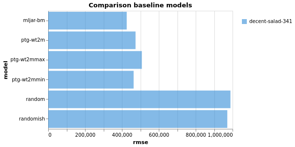
Still good to see that the PTG is still a good predictor, but the model output by mljar is doing a great job.

Hyperparameter optimization with hyperopt

In model development, executing grid search to find the right set of parameters of a model can time, and there are various approaches to navigate in parameters space that can be used:

Full grid search: testing all the sets of parameters in the parameters space (not time efficient)
Randomized search: testing a specific amount of parameters selected randomly in the space (time-efficient, but missing opportunities)

These approaches are very standard and working great, but sometimes you have some time constraints to do some experiments, and at this moment, a library like hyperopt can be used.

This package aims to use the Bayesian method to optimize a loss function (in this case, based on the rmse) by tweaking parameters in specific directions. You can find more details in this process here:

A paper that is behind the TPE approaches used in the hyperopt package
A general explanation of the bayesian process to do hyperparameter tuning made by Will Koehrsen

In the case of the prediction of the electrical consumption, there is the notebookbuilt based on the documentation of the package, and that is computing research on 100 iterations for a random forest regressor.

My research didn’t bring an excellent model to build the baseline (that was not the goal).

From a professional point of view is working great, tested on some projects at work I have maybe some reserved when you are executing Spark application but still an excellent package to have on hand if you are time constraint for your research (this is not the only package that can do this, you can find ray tune for example).

Let’s go further on the explainability of the model.

Make your model more explainable with shapash

Another aspect that I add recently at work was working on my machine learning models’ explainability. My research led me to a package developed by the insurance company MAIF (I didn’t expect to write this in an article on my blog) called shapash.

This package offers the ability to build an explainer level on the top of the model to help explain the model’s explainability and the prediction output if we are going back to the case of my random forest regressor to predict the electrical consumption.

There is the notebook used for this exploration of shapash.

I am using the best model from hyperopt with all the features precomputed; from the scikit learn, you can easily extract the importance of the features in the model (and shapash is offering an excellent visualization).

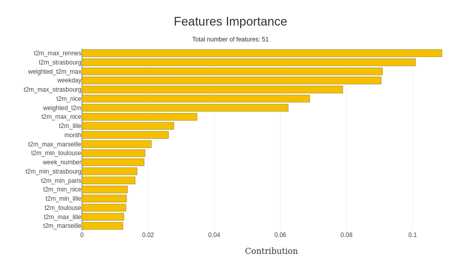
To notify that the predictor catches the importance of the day of the week and the temperatures in the modelization. An exciting feature of the package is looking at the specific value in the x dataset, like in this example; I focused on the weekend.

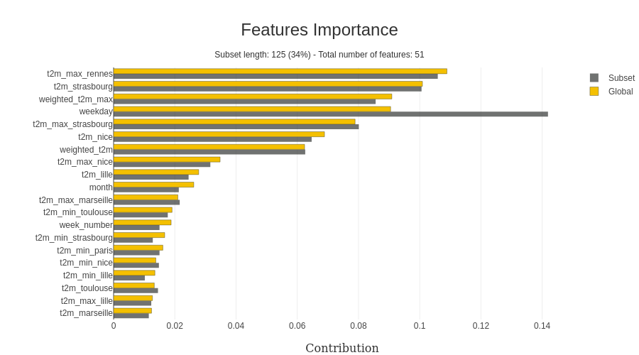
As we can see in this case, the day of the week is more important than on the previous representation. Another helpful feature if you want to dig on the impact of the value directly of a specific feature, contribution plot can be designed by the package (there is an example).

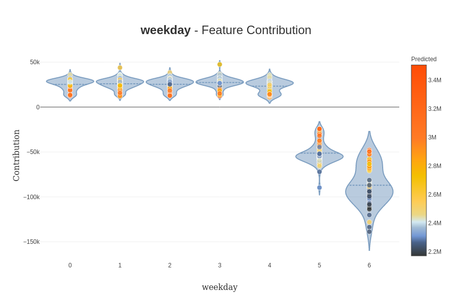
(still a good representation of the impact of the weekend on the prediction).

All this evaluation of the impact is impacted by the framework used behind the hood to evaluate this impact. Currently, two frameworks can be used :

SHAP: that is using Shapley values to build the impact of the features on a prediction; there is a good article that is illustrating this package
LIME: Another approach not based on Shapley values, more details here

If you are interested in model interpretability, you should consider Christoph Molnar’s work. He is doing an excellent job on this topic (he is behind a library called rulefit that can be useful for building baseline models).

To conclude on this package, the explainability can be applied directly at the prediction level with the ability for a specific prediction to have more details on it; there is a representation of the explainability for a prediction.

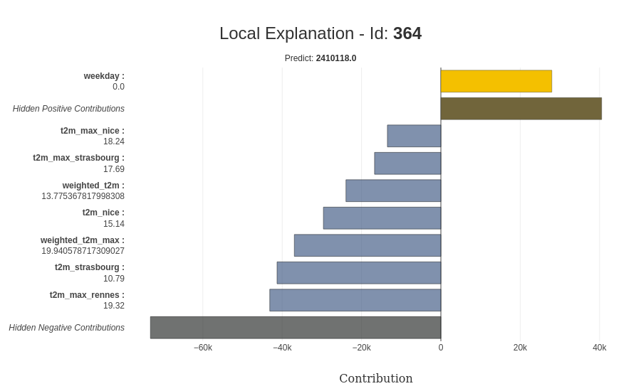
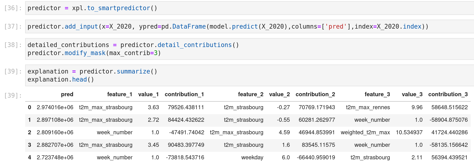
A cool feature is that this explainer element can be saved and be used on a predictor object for live prediction; there is an example on the data of 2020.

Other features could be helpful for you (like the little web app or the preprocessing of the elements), so I will strongly invite you to play with it (and look at the website of the open-source projects of MAIF here they are doing cool stuff).

Let’s go now on the evaluation of the drifting of the model and data.

Evaluate your data and model with evidently

Another project that I am working on at work is the monitoring of ml pipelines. I am mainly focusing my work on model drifting. In my feed, thanks to one of my colleagues, I saw this package that is developing an open-source library around data model drifting called evidently.

There is a company behind this package, but it is an open-source tool; you can hear one of the co-founders in this datacast; the package is quite simple to use. As I said previously, focus on drifting data and models, you can find the experimentation in this notebook.

Let’s dive into the data report; the previous notebook produces an example; the idea of this is to make the comparison between a referential dataset (in this case, the training set) versus another dataset (in this case, the year 2020) and see if there is a lot of divergences (that could explain the variation of the model in the prediction). Finally, there is a screenshot of the report produced.

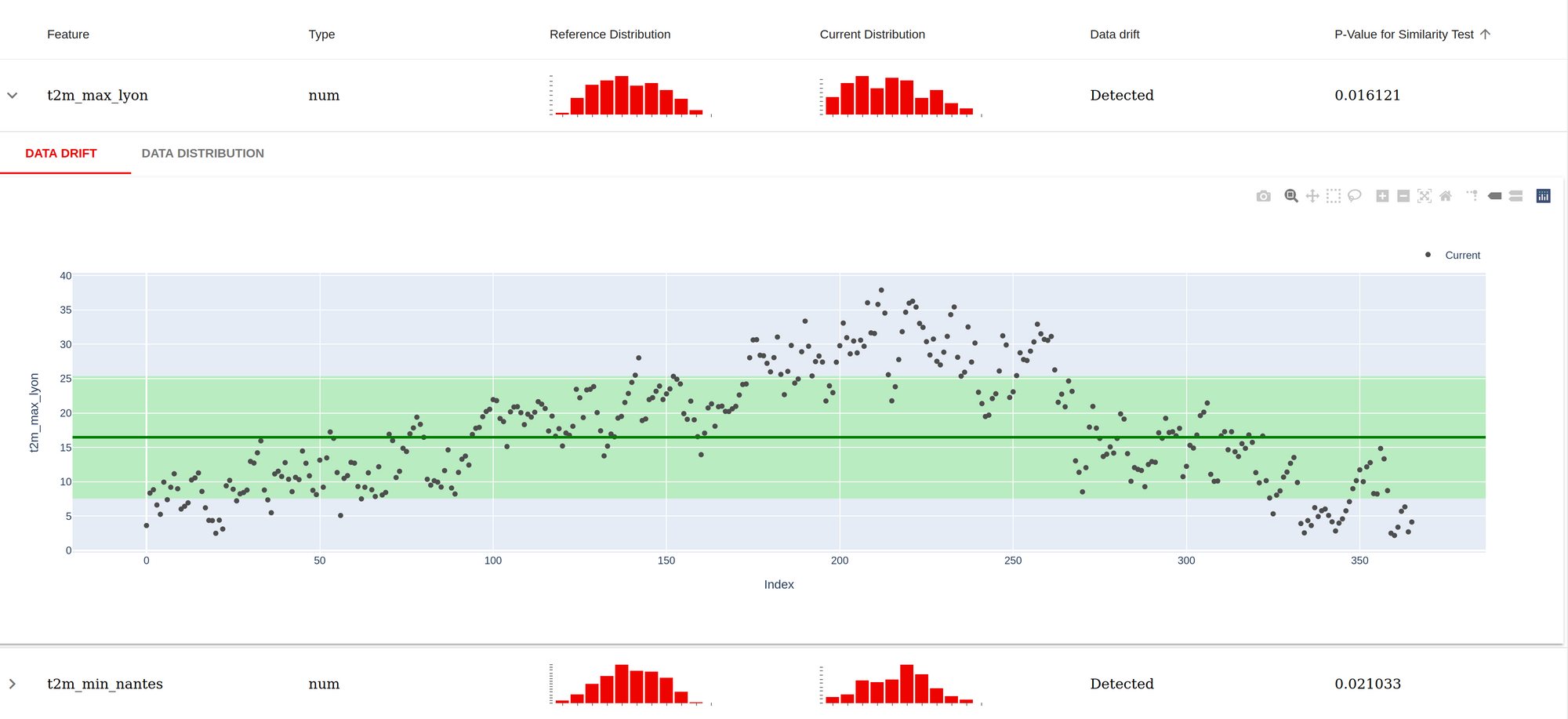
For each feature used in the model, there is an evaluation made in a similarity test between the reference data set and the current dataset (if the p-value is inferior to 0.05, there is something), as expected the temperature looks different, it’s expected as there are five years of data in the reference dataset versus one year of data). There are also a few graphs to dive a little bit more into the datasets.

The model report is similar, but the report is more evolved; there is an example here. The critical points on this report are:

The traditional evaluation metrics for a regression problem are displayed at the top.
Comparison on multiple plots on the prediction versus the actual values
The distinction between over and underestimations

The output of this reporting is not limited to an HTML file; it can be extracted in a JSON format.

This package is recent, but there are many good visualization and habits in it. Hence, I advise people to look at it (it’s not limited to regression work for classification, too) because it can inspire them for their dashboards (or maybe feed it).

Be more efficient to build your exploration pipeline with weights and biases

Finally, on this exploration, I tested another package called weights and biases that makes a lot of noise in the ML world (and for a good reason called weights and biases. This package is part of the package to help data scientists handle the monitoring of ml experiments easily and help them go to production.

One of the first aspects of the package is log information; you can log various elements from data, model, table or models. There is a quick snapshot of a code to version a dataframe and a model (load too).

# Log a dataframe
wandb.init(project='french_electrical_consumption', entity='jmdaignan')
data = [[row['model'], row['rmse']] for idx, row in dfp_evaluation_metrics.iterrows()]
table = wandb.Table(data=data, columns = ["model", "rmse"])
wandb.log({"comparison_baseline" : wandb.plot.bar(table, "model", "rmse", title="Comparison baseline models")})

# Log a model
run = wandb.init(project='french_electrical_consumption', entity='jmdaignan')

trained_model_artifact = wandb.Artifact('best_model_hyperopt', type='model', description='Best model from the hyperopt')

file_model = './data/model.pkl'
with open(file_model, 'wb') as file:
    pickle.dump(model, file)
trained_model_artifact.add_file(file_model)

run.log_artifact(trained_model_artifact)

# Load a model
run = wandb.init(project='french_electrical_consumption', entity='jmdaignan')
model_at = run.use_artifact('best_model_hyperopt:latest')
model_dir = model_at.download()
#model_dir = './data'
with open(model_dir + '/model.pkl', 'rb') as file:
    model = pickle.load(file)

This feature is very familiar in this kind of package ( as you can see in my article on mlflow). Still, one of the advantages is that you can use these artifacts in a nice UI to design graphs with data and write reports in a medium style.

A remarkable feature of this UI is monitoring the machine’s performance that is running the experiments.

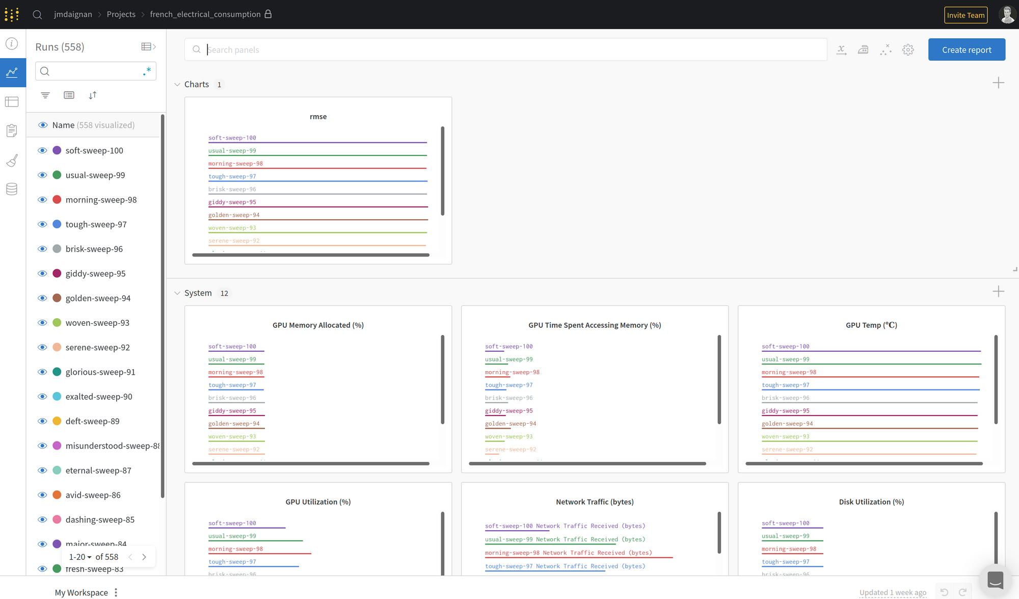
Another feature that I found very interesting is the sweep feature mixing hyperopt vision for the computation and a very nice interface. You can find the experiment in this notebook, but there is a screenshot of the UI.

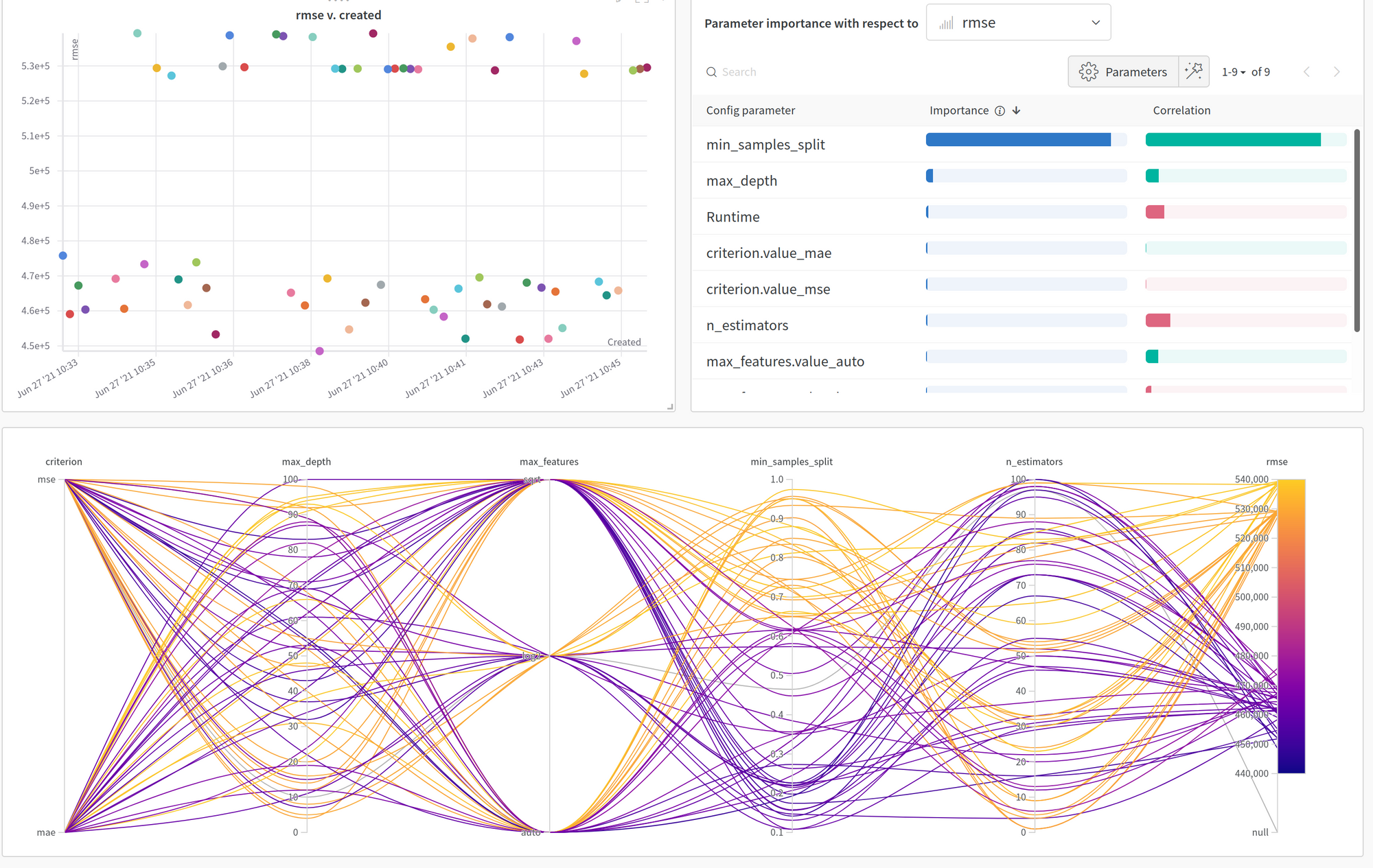
The UI is easy to understand using the parallel coordinates plot to study the impact of the parameters on the loss to optimize. But the remarkable feature that I like on this UI is the importance/ correlation graphs at the top right; for the importance of the parameters on the evolution of the loss, you can find the details on their approaches in this article.

Globally, weights and biases are an excellent package for monitoring; I am maybe not a big fan of the fact there is no experiment layer on a project (project> experiment > runs could be better for me), but it’s very efficient. I will just maybe highlight that for professional usage; a license needs to be paid per user, so be ready (but in the function of your ml teams configuration could be worth it)

Extra: Interface pandas with AWS storages easily with data wrangler

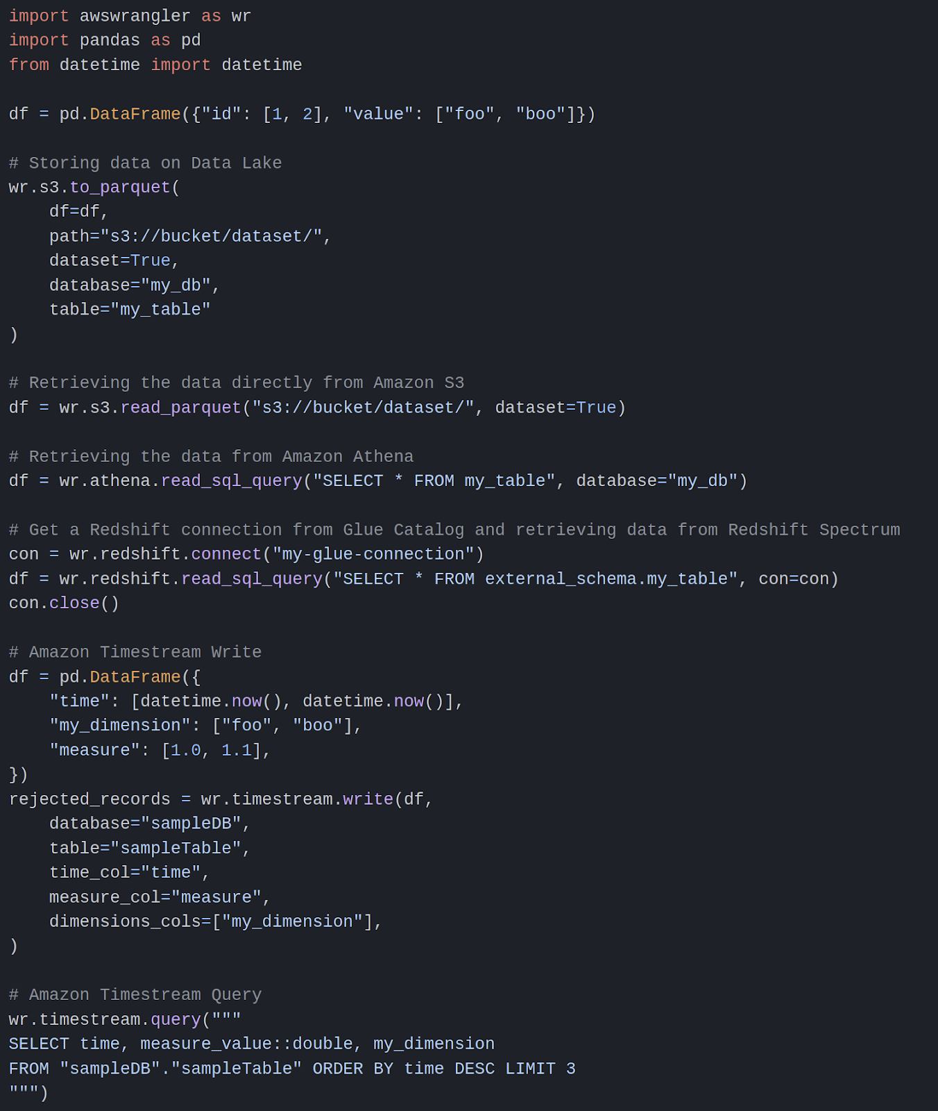
There is a package that I didn’t use in this project, but I wanted to share it here because I found it very useful. There is a package of AWS that is helping to connect pandas dataframe with AWS storage (there is a snapshot of code to interface pandas with various AWS services)

Nothing really to say; if your machine has enough rights on the AWS services to call, it’s an excellent package to do the interface (for me,.he only drawbacks are the missing reading capability on dynamodb).

Conclusion

I hope this article gave you the curiosity to test these packages because they can make your life easier in your ML/DS day-to-day work.

Kickstart a big data project with AWS EMR and Pyspark

Evaluation of recommender systems (metrics and baseline models)